PSM倾向性得分匹配
·
Xiebro
背景目标
- A为对照组,B为实验组;
- A组和B组样本的特征分布不均匀,无法直接使用随机对照实验中的显著性检验;
- 利用PSM方法消除A组与B组样本的差异(只能在已知特征范围内),近似地创造随机对照实验环境。
模拟数据集
set.seed(123)

# generate group A
n_a <- 1500
dat_A <-
  data.frame(age = rnorm(n_a, mean = 50, sd = 10),
             gender = sample(c("Male", "Female"), size = n_a, replace = TRUE),
             health = rnorm(n_a, mean = 0, sd = 1),
             income = rnorm(n_a, mean = 50000, sd = 10000),
             education = sample(c("High School", "Bachelor's Degree", "Master's Degree", "PhD"), size = n_a, replace = TRUE),
             treatment = rep(0, n_a)  # A组均未参与实验
  )

# generate group B
n_b <- 500
dat_B <-
  data.frame(age = rnorm(n_b, mean = 47, sd = 12),
             gender = sample(c("Male", "Female"), size = n_b, replace = TRUE),
             health = rnorm(n_b, mean = 0.2, sd = 1),
             income = rnorm(n_b, mean = 52000, sd = 12000),
             education = sample(c("Bachelor's Degree", "Master's Degree", "PhD"), size = n_b, replace = TRUE),
             treatment = rep(1, n_b)  # B组全部参与实验
  )

dat <- rbind(dat_A, dat_B)

head(dat, 5)
##        age gender     health   income         education treatment
## 1 44.39524 Female -1.2533359 35767.06   Master's Degree         0
## 2 47.69823   Male -0.1113319 60223.04               PhD         0
## 3 65.58708 Female -1.4128135 56878.15               PhD         0
## 4 50.70508 Female -1.9829539 46925.45       High School         0
## 5 51.29288   Male  0.7835954 49802.51 Bachelor's Degree         0
数据现状
AB组样本特征差异对比
library(tableone)

strt <- CreateTableOne(data = dat,
                       vars = names(dat),
                       strata='treatment',
                       test = TRUE)

print(strt, smd = TRUE)
##                        Stratified by treatment
##                         0                  1                   p      test
##   n                         1500                500
##   age (mean (SD))          50.19 (9.92)       46.61 (12.33)    <0.001
##   gender = Male (%)          716 (47.7)         234 (46.8)      0.756
##   health (mean (SD))       -0.01 (1.00)        0.19 (0.95)     <0.001
##   income (mean (SD))    49841.81 (9860.18) 51911.59 (12187.28) <0.001
##   education (%)                                                <0.001
##      Bachelor's Degree       382 (25.5)         177 (35.4)
##      High School             409 (27.3)           0 ( 0.0)
##      Master's Degree         373 (24.9)         159 (31.8)
##      PhD                     336 (22.4)         164 (32.8)
##   treatment (mean (SD))     0.00 (0.00)        1.00 (0.00)     <0.001
##                        Stratified by treatment
##                         SMD
##   n
##   age (mean (SD))        0.321
##   gender = Male (%)      0.019
##   health (mean (SD))     0.201
##   income (mean (SD))     0.187
##   education (%)          0.868
##      Bachelor's Degree
##      High School
##      Master's Degree
##      PhD
##   treatment (mean (SD))    Inf
PSM匹配
由上图可见,AB组样本中的age、health、income、education特征存在显著性差异,接下来基于PSM方法将AB组样本特征拉齐(在A中找到与B最相似的样本子集)
library(MatchIt)
psm_matchit <-
  matchit(data = dat,
          treatment ~ age + gender + health + income + education,
          method = 'nearest', # 近邻匹配
          ratio = 1, # 匹配数量
          replace = F, # 不放回
          caliper = 0.2)

summary(psm_matchit)
##
## Call:
## matchit(formula = treatment ~ age + gender + health + income +
##     education, data = dat, method = "nearest", replace = F, caliper = 0.2,
##     ratio = 1)
##
## Summary of Balance for All Data:
##                            Means Treated Means Control Std. Mean Diff.
## distance                          0.3411        0.2196          1.2271
## age                              46.6085       50.1949         -0.2908
## genderFemale                      0.5320        0.5227          0.0187
## genderMale                        0.4680        0.4773         -0.0187
## health                            0.1895       -0.0062          0.2057
## income                        51911.5857    49841.8071          0.1698
## educationBachelor's Degree        0.3540        0.2547          0.2077
## educationHigh School              0.0000        0.2727         -0.7070
## educationMaster's Degree          0.3180        0.2487          0.1489
## educationPhD                      0.3280        0.2240          0.2215
##                            Var. Ratio eCDF Mean eCDF Max
## distance                       0.4224    0.2165   0.3153
## age                            1.5460    0.0849   0.1580
## genderFemale                        .    0.0093   0.0093
## genderMale                          .    0.0093   0.0093
## health                         0.9146    0.0591   0.1113
## income                         1.5277    0.0584   0.1287
## educationBachelor's Degree          .    0.0993   0.0993
## educationHigh School                .    0.2727   0.2727
## educationMaster's Degree            .    0.0693   0.0693
## educationPhD                        .    0.1040   0.1040
##
## Summary of Balance for Matched Data:
##                            Means Treated Means Control Std. Mean Diff.
## distance                          0.3362        0.3343          0.0190
## age                              47.0493       47.7105         -0.0536
## genderFemale                      0.5255        0.5153          0.0204
## genderMale                        0.4745        0.4847         -0.0204
## health                            0.1714        0.1749         -0.0037
## income                        51718.5638    52309.7730         -0.0485
## educationBachelor's Degree        0.3503        0.3523         -0.0043
## educationHigh School              0.0000        0.0000          0.0000
## educationMaster's Degree          0.3238        0.3218          0.0044
## educationPhD                      0.3259        0.3259          0.0000
##                            Var. Ratio eCDF Mean eCDF Max Std. Pair Dist.
## distance                       1.0644    0.0022   0.0326          0.0208
## age                            1.3452    0.0305   0.0611          0.6766
## genderFemale                        .    0.0102   0.0102          0.9510
## genderMale                          .    0.0102   0.0102          0.9510
## health                         0.9111    0.0140   0.0489          1.0292
## income                         1.6186    0.0483   0.0937          0.8530
## educationBachelor's Degree          .    0.0020   0.0020          0.9838
## educationHigh School                .    0.0000   0.0000          0.0000
## educationMaster's Degree            .    0.0020   0.0020          0.9403
## educationPhD                        .    0.0000   0.0000          0.4399
##
## Sample Sizes:
##           Control Treated
## All          1500     500
## Matched       491     491
## Unmatched    1009       9
## Discarded       0       0
平衡性检验
- SMD < 0.1?
library(cobalt)
bal.tab(psm_matchit,m.threshold = 0.1, un = FALSE)
## Balance Measures
##                                 Type Diff.Adj    M.Threshold
## distance                    Distance   0.0190 Balanced, <0.1
## age                          Contin.  -0.0536 Balanced, <0.1
## gender_Male                   Binary  -0.0102 Balanced, <0.1
## health                       Contin.  -0.0037 Balanced, <0.1
## income                       Contin.  -0.0485 Balanced, <0.1
## education_Bachelor's Degree   Binary  -0.0020 Balanced, <0.1
## education_High School         Binary   0.0000 Balanced, <0.1
## education_Master's Degree     Binary   0.0020 Balanced, <0.1
## education_PhD                 Binary   0.0000 Balanced, <0.1
##
## Balance tally for mean differences
##                    count
## Balanced, <0.1         9
## Not Balanced, >0.1     0
##
## Variable with the greatest mean difference
##  Variable Diff.Adj    M.Threshold
##       age  -0.0536 Balanced, <0.1
##
## Sample sizes
##           Control Treated
## All          1500     500
## Matched       491     491
## Unmatched    1009       9
- 匹配与未匹配样本的倾向性得分差异
plot(psm_matchit, type = "jitter")
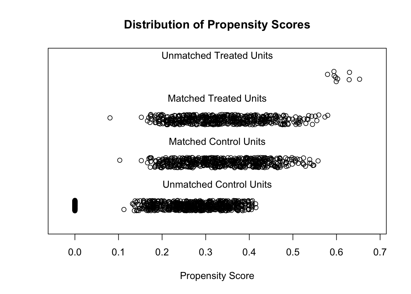
## To identify the units, use first mouse button; to stop, use second.
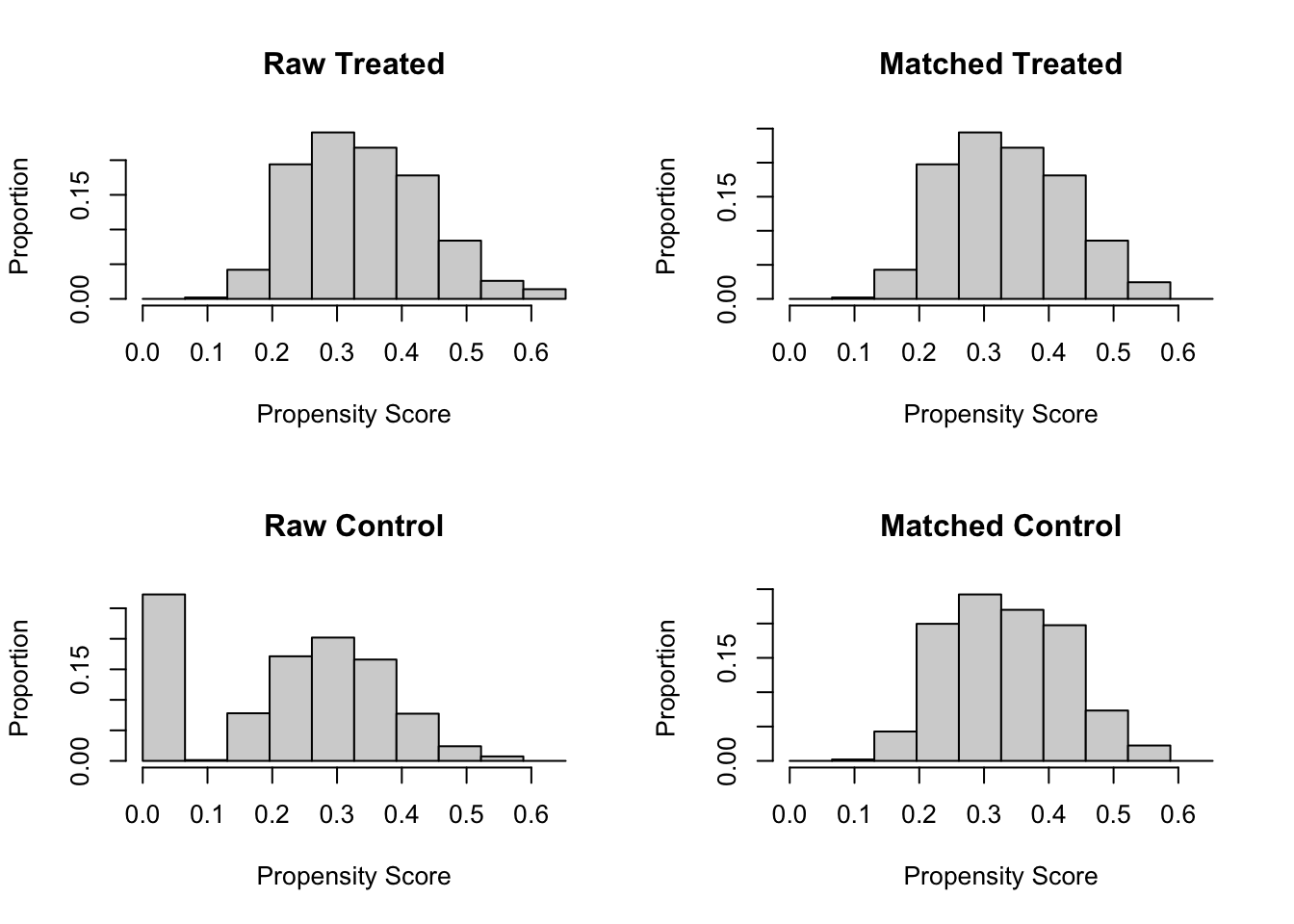
- 匹配与未匹配样本的倾向性得分分布
plot(psm_matchit, type = "hist")
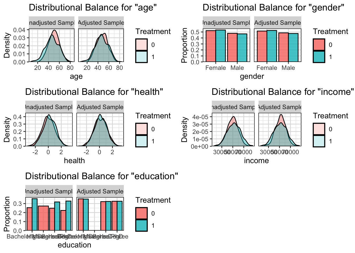
- 匹配前后的特征分布对比
cowplot::plot_grid(
  ncol = 2,
  bal.plot(psm_matchit, var.name = "age", which = "both", grid = TRUE),
  bal.plot(psm_matchit, var.name = "gender", which = "both", grid = TRUE),
  bal.plot(psm_matchit, var.name = "health", which = "both", grid = TRUE),
  bal.plot(psm_matchit, var.name = "income", which = "both", grid = TRUE),
  bal.plot(psm_matchit, var.name = "education", which = "both", grid = TRUE))
匹配后样本
- 获取结果样本
psm_matchit_dat <-
  match.data(psm_matchit) |>
  as.data.frame()
- 结果样本AB差异
strt <-
  CreateTableOne(data = psm_matchit_dat,
                 vars = names(dat),
                 strata='treatment',
                 test = TRUE)

print(strt, smd = TRUE)
##                        Stratified by treatment
##                         0                  1                   p      test
##   n                          491                491
##   age (mean (SD))          47.71 (10.31)      47.05 (11.96)     0.354
##   gender = Male (%)          238 (48.5)         233 (47.5)      0.798
##   health (mean (SD))        0.17 (0.99)        0.17 (0.95)      0.955
##   income (mean (SD))    52309.77 (9536.96) 51718.56 (12133.35)  0.396
##   education (%)                                                 0.997
##      Bachelor's Degree       173 (35.2)         172 (35.0)
##      Master's Degree         158 (32.2)         159 (32.4)
##      PhD                     160 (32.6)         160 (32.6)
##   treatment (mean (SD))     0.00 (0.00)        1.00 (0.00)     <0.001
##                        Stratified by treatment
##                         SMD
##   n
##   age (mean (SD))        0.059
##   gender = Male (%)      0.020
##   health (mean (SD))     0.004
##   income (mean (SD))     0.054
##   education (%)          0.005
##      Bachelor's Degree
##      Master's Degree
##      PhD
##   treatment (mean (SD))    Inf