DID平行趋势检验
·
Xiebro
数据集
采用普林斯顿大学OscarTorres-Reyna教授构建的DID虚拟数据集进行演示分析,该数据集假设1994年在E、F、G三个国家实施了一项政策,并与相似的A、B、C、D四个国家为控制组。数据集共包含country、year、y、x1、 x2、 x3、 opinion 7个变量,其中y为被解释变量,x1-x3为连续型的自变量,opinion为分类型自变量。
library(dplyr)
dat <- haven::read_dta("http://dss.princeton.edu/training/Panel101.dta")
dat |> glimpse()
## Rows: 70
## Columns: 9
## $ country <dbl+lbl> 1, 1, 1, 1, 1, 1, 1, 1, 1, 1, 2, 2, 2, 2, 2, 2, 2, 2, 2, 2…
## $ year    <dbl> 1990, 1991, 1992, 1993, 1994, 1995, 1996, 1997, 1998, 1999, 19…
## $ y       <dbl> 1342787840, -1899660544, -11234363, 2645775360, 3008334848, 32…
## $ y_bin   <dbl> 1, 0, 0, 1, 1, 1, 1, 1, 1, 1, 0, 0, 0, 1, 1, 1, 1, 1, 0, 0, 0,…
## $ x1      <dbl> 0.27790365, 0.32068470, 0.36346573, 0.24614404, 0.42462304, 0.…
## $ x2      <dbl> -1.1079559, -0.9487200, -0.7894840, -0.8855330, -0.7297683, -0…
## $ x3      <dbl> 0.28255358, 0.49253848, 0.70252335, -0.09439092, 0.94613063, 1…
## $ opinion <dbl+lbl> 1, 3, 3, 3, 3, 1, 3, 1, 3, 4, 2, 1, 2, 4, 3, 4, 1, 3, 2, 4…
## $ op      <dbl> 1, 0, 0, 0, 0, 1, 0, 1, 0, 0, 1, 1, 1, 0, 0, 0, 1, 0, 1, 0, 1,…
DID回归模型
library(estimatr)
dat <-
  dat %>%
  # 生成实验期变量,1994年赋值为1,否则为0
  mutate(time = (year >= 1994) & (!is.na(year)),
         # 生成实验组变量,前4个国家为控制组,赋值为0,否则为1
         treated = (country > 4) & (!is.na(country)),
         # 生成交互项
         did = time * treated)

lm_robust(y ~ time + treated + did + x1 + x2 + x3 + factor(opinion), data = dat)
##                     Estimate Std. Error     t value   Pr(>|t|)    CI Lower
## (Intercept)        136849585  915761890  0.14943796 0.88170924 -1694946928
## timeTRUE          2169928587  944783027  2.29674806 0.02513936   280081156
## treatedTRUE       2536658512 1168802696  2.17030515 0.03395261   198705025
## did              -3188869350 1532703396 -2.08055215 0.04175287 -6254732616
## x1                 750264236  947661865  0.79170036 0.43165425 -1145341729
## x2                  13769207  322645914  0.04267591 0.96610159  -631618713
## x3                -221188166  283777634 -0.77944186 0.43878316  -788827950
## factor(opinion)2 -1874190600 1414901918 -1.32460814 0.19032440 -4704415825
## factor(opinion)3  1080043365  841203885  1.28392579 0.20410396  -602614934
## factor(opinion)4  -314666706  837453259 -0.37574241 0.70843362 -1989822636
##                    CI Upper DF
## (Intercept)      1968646099 60
## timeTRUE         4059776018 60
## treatedTRUE      4874611998 60
## did              -123006085 60
## x1               2645870200 60
## x2                659157127 60
## x3                346451618 60
## factor(opinion)2  956034624 60
## factor(opinion)3 2762701665 60
## factor(opinion)4 1360489223 60
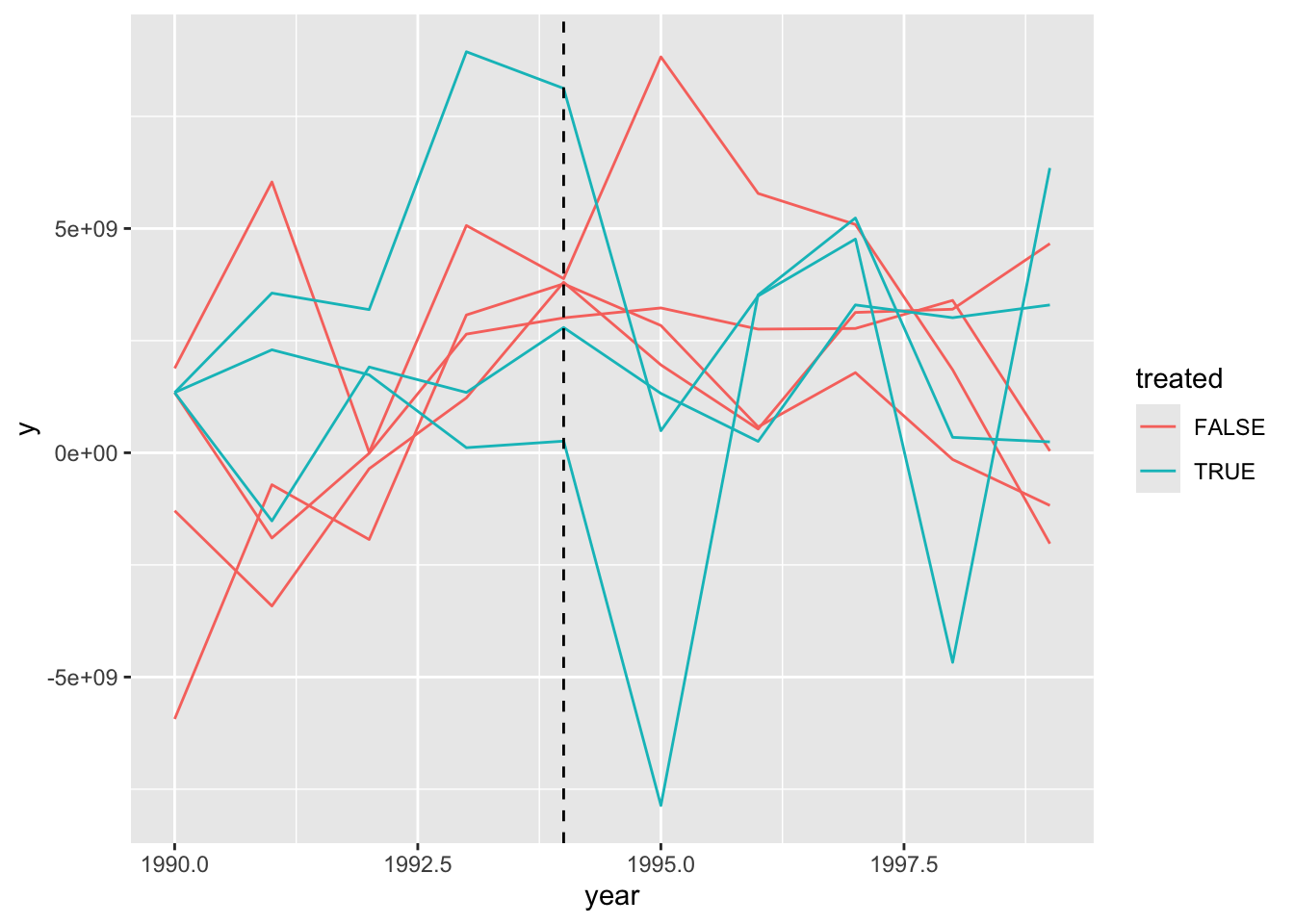
平行趋势检验
平行趋势检验的主要目的是验证在政策实施前,实验组和控制组是否存在显著性差异,即与实验组特征相似才可以作为控制组。
方法一:趋势观察法
library(ggplot2)
dat %>%
  select(year, y, country, treated) %>%
  ggplot(aes(x = year, y = y, group = country)) +
  geom_line(aes(group = country, col = treated)) +
  geom_vline(aes(xintercept = 1994), lty = "dashed", size = .5)
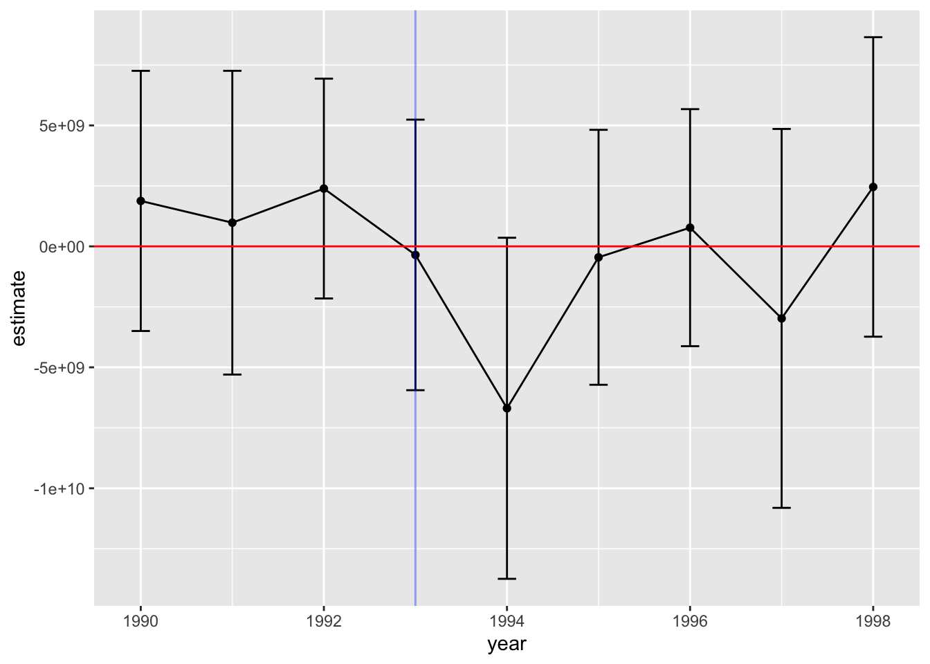
方法二:事件研究法
即生成年份的虚拟变量后于treat变量做交互项,然后进行回归。如果政策实施前,每个交互项的系数不显著的异于0,则表示实验组与对照组不存在显著性差异。
# 事件研究法
dat <-
  dat |>
  mutate(year = factor(year),
         country = factor(country))

# 将政策前第一期(1993年)作为基准组
X <-
  model.matrix(y ~ country + year + year:treated, data = dat) |>
  as_tibble() |>
  select(-1, -`year1993:treatedTRUE`) # 避免多重共线性问题

fit <-
  lm_robust(dat$y ~ ., data = X) |>
  tidy()

print(fit)
##                      term    estimate  std.error   statistic     p.value
## 1             (Intercept) -1004008065 1402457934 -0.71589175 0.477756796
## 2                country2 -1514179010  681334421 -2.22237269 0.031327773
## 3                country3  -383469504  901301281 -0.42546207 0.672527761
## 4                country4  1912414982 1004283630  1.90425785 0.063281799
## 5                country5  -805089473 2247093543 -0.35828036 0.721808836
## 6                country6  2031087929 2515770746  0.80734222 0.423716318
## 7                country7   177750362 2208439844  0.08048685 0.936206953
## 8                year1991  1002945936 2121458148  0.47276254 0.638667653
## 9                year1992   427838696 1381280329  0.30974067 0.758188010
## 10               year1993  4003056960 1451134803  2.75857002 0.008362949
## 11               year1994  4615611360 1500563418  3.07591889 0.003563444
## 12               year1995  5213781216 1664447129  3.13244027 0.003045850
## 13               year1996  3411949032 1450700360  2.35193230 0.023112337
## 14               year1997  4194826080 1306329779  3.21115399 0.002442031
## 15               year1998  3075285908 1588038874  1.93653062 0.059097606
## 16               year1999  1376036696 2330887963  0.59034871 0.557910106
## 17 `year1990:treatedTRUE`  1878879632 2669980342  0.70370542 0.485241725
## 18 `year1991:treatedTRUE`   978954411 3117370139  0.31403214 0.754947866
## 19 `year1992:treatedTRUE`  2389146024 2255634352  1.05919030 0.295165568
## 20 `year1994:treatedTRUE`  -353480357 2776486067 -0.12731213 0.899260572
## 21 `year1995:treatedTRUE` -6693704891 3500326459 -1.91230874 0.062214974
## 22 `year1996:treatedTRUE`  -451797160 2616161141 -0.17269470 0.863665814
## 23 `year1997:treatedTRUE`   773399515 2432758346  0.31791054 0.752023424
## 24 `year1998:treatedTRUE` -2977579631 3888349384 -0.76576957 0.447811584
## 25 `year1999:treatedTRUE`  2456562845 3073685394  0.79922391 0.428359108
##        conf.low  conf.high df outcome
## 1   -3828703341 1820687212 45   dat$y
## 2   -2886456977 -141901043 45   dat$y
## 3   -2198783469 1431844460 45   dat$y
## 4    -110316080 3935146043 45   dat$y
## 5   -5330968193 3720789247 45   dat$y
## 6   -3035934457 7098110314 45   dat$y
## 7   -4270275812 4625776537 45   dat$y
## 8   -3269890109 5275781981 45   dat$y
## 9   -2354202695 3209880088 45   dat$y
## 10   1080321435 6925792485 45   dat$y
## 11   1593321494 7637901226 45   dat$y
## 12   1861412613 8566149819 45   dat$y
## 13    490088520 6333809544 45   dat$y
## 14   1563742845 6825909315 45   dat$y
## 15   -123188570 6273760386 45   dat$y
## 16  -3318612649 6070686041 45   dat$y
## 17  -3498736823 7256496087 45   dat$y
## 18  -5299751350 7257660171 45   dat$y
## 19  -2153934769 6932226816 45   dat$y
## 20  -5945610355 5238649640 45   dat$y
## 21 -13743724274  356314493 45   dat$y
## 22  -5721016180 4817421860 45   dat$y
## 23  -4126427315 5673226344 45   dat$y
## 24 -10809117303 4853958042 45   dat$y
## 25  -3734157324 8647283015 45   dat$y
-
上述结果显示,1991至1993的交互项均不显著,表示实验组和控制组在政策实施前并无显著差异;
-
其次,1994年政策实施后,仅有1995的系数显著,表明政策效应仅出现在政策实施后一年,1996年及以后实验组和控制组未受到政策的影响。
# 可视化:结果系数和置信区间
fit %>%
  tail(9) |>
  mutate(year = 1990 + 0:(n()-1)) |>
  ggplot(aes(x = year, y = estimate)) +
  geom_point() +
  geom_line() +
  geom_errorbar(aes(ymin = conf.low, ymax = conf.high, width = .2))  +
  geom_vline(aes(xintercept = 1993), color = "blue", alpha = .4) +
  geom_hline(aes(yintercept = 0), color = "red")
安慰剂检验
-
政策的实施确实产生了政策效应,且政策实施前实验组和控制组不存在显著性差异,但是通过DID估计出的政策效应是否受其他政策或因素的影响是未知的,因此需要进行安慰剂检验;
-
最常用的方法就是将研究样本缩小至政策实施前,并随机设定一个政策实施年份;
-
样本是1990-1999年,政策实施年份为1994年,故本次安慰剂假设政策时间发生在1994年以前。将研究样本设定在1990-1994间,并将政策年份设定在1992年。
dat_new <-
  dat |>
  mutate(year = as.character(year) |> as.numeric()) |>
  filter(year <= 1994) |>
  mutate(time_new = (year >= 1992),
         did_new = time_new * treated)

fit_new <-
  lm_robust(y ~ time_new + treated + did_new + x1 + x2 + x3 + factor(opinion),
            dat = dat_new)

summary(fit_new)
##
## Call:
## lm_robust(formula = y ~ time_new + treated + did_new + x1 + x2 +
##     x3 + factor(opinion), data = dat_new)
##
## Standard error type:  HC2
##
## Coefficients:
##                    Estimate Std. Error  t value Pr(>|t|)   CI Lower  CI Upper
## (Intercept)       1.180e+08  1.264e+09  0.09334  0.92638 -2.486e+09 2.721e+09
## time_newTRUE      2.043e+09  1.588e+09  1.28664  0.21001 -1.227e+09 5.314e+09
## treatedTRUE       2.797e+09  1.395e+09  2.00494  0.05591 -7.616e+07 5.670e+09
## did_new          -7.945e+07  1.968e+09 -0.04038  0.96811 -4.132e+09 3.973e+09
## x1               -4.839e+08  1.444e+09 -0.33499  0.74043 -3.459e+09 2.491e+09
## x2               -1.443e+08  5.602e+08 -0.25753  0.79888 -1.298e+09 1.009e+09
## x3               -1.055e+09  9.381e+08 -1.12465  0.27142 -2.987e+09 8.770e+08
## factor(opinion)2 -1.852e+09  1.528e+09 -1.21158  0.23700 -5.000e+09 1.296e+09
## factor(opinion)3  1.366e+09  1.615e+09  0.84564  0.40577 -1.960e+09 4.692e+09
## factor(opinion)4  2.756e+07  1.296e+09  0.02127  0.98320 -2.641e+09 2.696e+09
##                  DF
## (Intercept)      25
## time_newTRUE     25
## treatedTRUE      25
## did_new          25
## x1               25
## x2               25
## x3               25
## factor(opinion)2 25
## factor(opinion)3 25
## factor(opinion)4 25
##
## Multiple R-squared:  0.3519 ,	Adjusted R-squared:  0.1186
## F-statistic: 1.824 on 9 and 25 DF,  p-value: 0.1136
did_new的系数为负,但不显著,表明可以排除其他潜在的不可观测因素的影响,即模型估计出的政策效应是稳健的。