缺失值填充
·
xiebro
library(tidyverse)
library(titanic)
library(patchwork)
seed <- 42
set.seed(seed)
演示数据
演示对Age列进行插值
dat <- titanic::titanic_train
glimpse(dat)
## Rows: 891
## Columns: 12
## $ PassengerId <int> 1, 2, 3, 4, 5, 6, 7, 8, 9, 10, 11, 12, 13, 14, 15, 16, 17,…
## $ Survived    <int> 0, 1, 1, 1, 0, 0, 0, 0, 1, 1, 1, 1, 0, 0, 0, 1, 0, 1, 0, 1…
## $ Pclass      <int> 3, 1, 3, 1, 3, 3, 1, 3, 3, 2, 3, 1, 3, 3, 3, 2, 3, 2, 3, 3…
## $ Name        <chr> "Braund, Mr. Owen Harris", "Cumings, Mrs. John Bradley (Fl…
## $ Sex         <chr> "male", "female", "female", "female", "male", "male", "mal…
## $ Age         <dbl> 22, 38, 26, 35, 35, NA, 54, 2, 27, 14, 4, 58, 20, 39, 14, …
## $ SibSp       <int> 1, 1, 0, 1, 0, 0, 0, 3, 0, 1, 1, 0, 0, 1, 0, 0, 4, 0, 1, 0…
## $ Parch       <int> 0, 0, 0, 0, 0, 0, 0, 1, 2, 0, 1, 0, 0, 5, 0, 0, 1, 0, 0, 0…
## $ Ticket      <chr> "A/5 21171", "PC 17599", "STON/O2. 3101282", "113803", "37…
## $ Fare        <dbl> 7.2500, 71.2833, 7.9250, 53.1000, 8.0500, 8.4583, 51.8625,…
## $ Cabin       <chr> "", "C85", "", "C123", "", "", "E46", "", "", "", "G6", "C…
## $ Embarked    <chr> "S", "C", "S", "S", "S", "Q", "S", "S", "S", "C", "S", "S"…
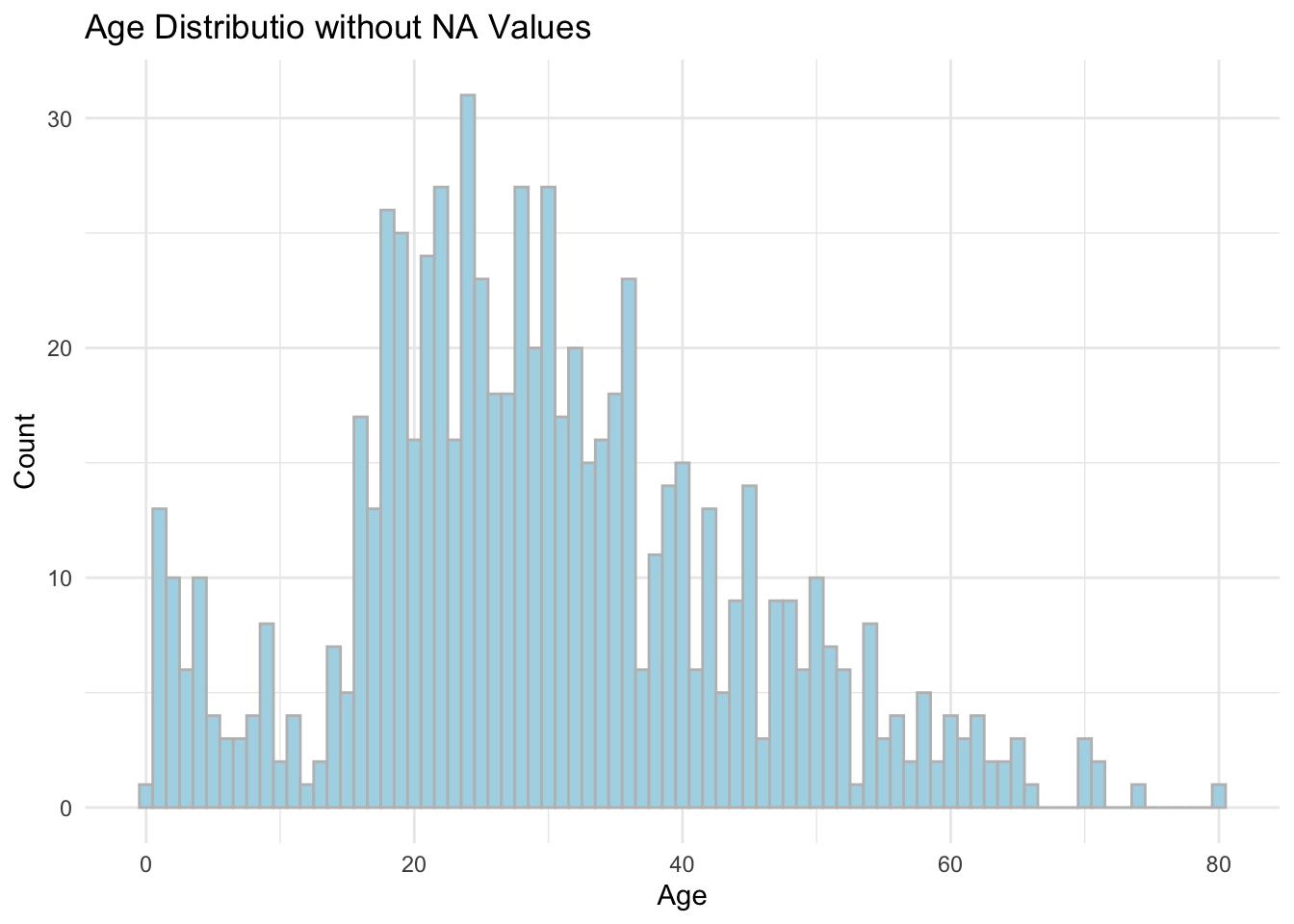
# 原始数据Age分布
dat %>%
  ggplot(aes(x = Age)) +
  geom_histogram(fill = "lightblue", col = "grey", binwidth = 1) +
  theme(axis.text.x = element_text(angle = 90)) +
  labs(
    title = "Age Distributio without NA Values",
    x = "Age",
    y = "Count"
  ) +
  theme_minimal()
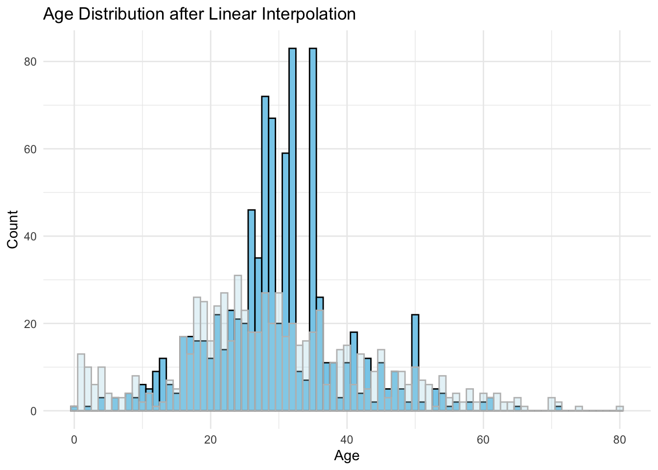
线性插值填充
library(zoo)
# 使用线性插值法填充NA值
dat %>%
  arrange(Age, Fare) %>%
  mutate(Age = na.approx(Age, x = Fare, na.rm = FALSE)) %>% # 以Fare列作为相关变量
  ggplot(aes(x = Age)) +
  geom_histogram(fill = "skyblue", color = "black", binwidth = 1) + # 插值后分布
  geom_histogram(data = dat, fill = "lightblue", col = "grey", alpha = 0.3, binwidth = 1) + # 插值前分布
  labs(
    title = "Age Distribution after Linear Interpolation",
    x = "Age",
    y = "Count"
  ) +
  theme_minimal()
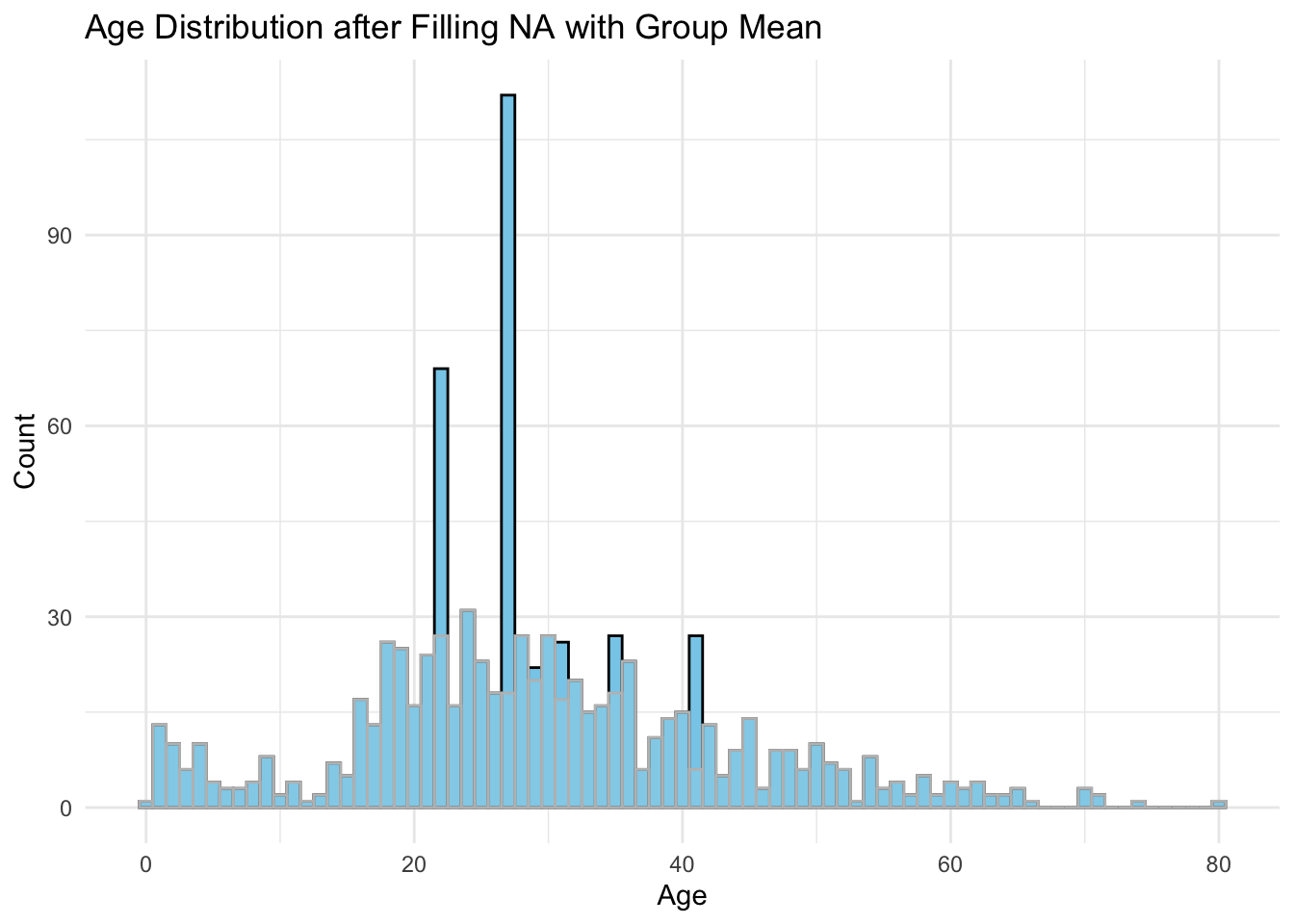
同类均值填充
# 使用同类均值填充NA值
dat %>%
  group_by(Sex, Pclass) %>%
  mutate(Age = ifelse(is.na(Age), mean(Age, na.rm = TRUE), Age)) %>%
  ungroup() %>%
  ggplot(aes(x = Age)) +
  geom_histogram(fill = "skyblue", color = "black", binwidth = 1) +
  geom_histogram(data = dat, fill = "lightblue", col = "grey", alpha = 0.3, binwidth = 1) +
  labs(
    title = "Age Distribution after Filling NA with Group Mean",
    x = "Age",
    y = "Count"
  ) +
  theme_minimal()
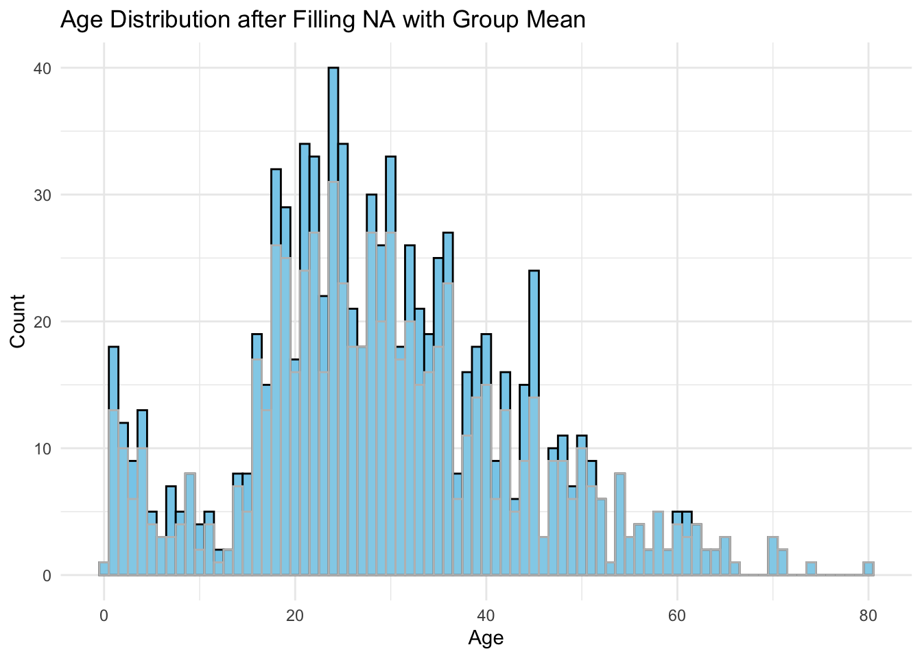
同类邻近值填充
# 分组排序后,使用邻近值填充
dat %>%
  arrange(PassengerId) %>%
  group_by(Sex, Pclass) %>%
  fill(Age, .direction = "updown") %>% # .direction可选参数:up/down/updown/downup
  ungroup() %>%
  ggplot(aes(x = Age)) +
  geom_histogram(fill = "skyblue", color = "black", binwidth = 1) +
  geom_histogram(data = dat, fill = "lightblue", col = "grey", alpha = 0.3, binwidth = 1) +
  labs(
    title = "Age Distribution after Filling NA with Group Mean",
    x = "Age",
    y = "Count"
  ) +
  theme_minimal()
模型预测值填充
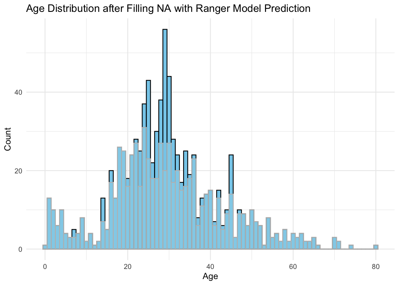
回归法
library(ranger)
# 构建随机森林预测模型
dat_age <-
  dat %>%
  select(Age, Pclass, Sex, Fare, Parch, SibSp) %>%
  mutate(Sex = as.factor(Sex))

known_age <- dat_age %>% filter(!is.na(Age)) # 已知年龄
unknown_age <- dat_age %>% filter(is.na(Age)) # 未知年龄

X_train <- known_age %>% select(-Age) # 训练集
y_train <- known_age$Age # 目标label

X_test <- unknown_age %>% select(-Age) # 测试集

# 训练随机森林模型
rfr <- ranger(Age ~ ., data = known_age, num.trees = 2000)

# 预测未知年龄
y_pred <- predict(rfr, X_test)$predictions

# 填充原缺失数据
dat_fill <-
  dat %>%
  mutate(Age = ifelse(is.na(Age), y_pred, Age))

dat_fill %>%
  ggplot(aes(x = Age)) +
  geom_histogram(fill = "skyblue", color = "black", binwidth = 1) +
  geom_histogram(data = dat, fill = "lightblue", col = "grey", alpha = 0.3, binwidth = 1) +
  labs(
    title = "Age Distribution after Filling NA with Ranger Model Prediction",
    x = "Age",
    y = "Count"
  ) +
  theme_minimal()
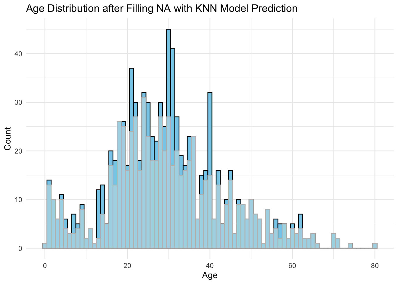
最近距离邻法(KNN)
library(VIM)
# 使用kNN进行缺失值插补
imp <- kNN(dat, variable = "Age", k = 5)

imp %>%
  ggplot(aes(x = Age)) +
  geom_histogram(fill = "skyblue", col = "black", binwidth = 1) +
  geom_histogram(data = dat, fill = "lightblue", col = "grey", binwidth = 1) +
  labs(
    title = "Age Distribution after Filling NA with KNN Model Prediction",
    x = "Age",
    y = "Count"
  ) +
  theme_minimal()
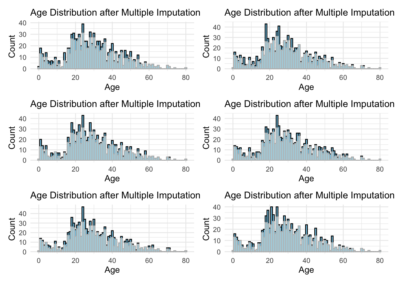
多重插补填充
library(mice)

# 使用 mice 进行多重插补
imp <- mice(titanic_train, m = 6, method = "pmm", seed = seed, printFlag = FALSE) # m 表示生成 m 个数据集

imp_dat <- complete(imp, 1)

1:6 %>%
  map(~ {
    complete(imp, .x)
  }) %>%
  map(~ {
    .x %>%
      ggplot(aes(x = Age)) +
      geom_histogram(fill = "skyblue", col = "black", binwidth = 1) +
      geom_histogram(data = dat, fill = "lightblue", col = "grey", binwidth = 1) +
      labs(
        title = "Age Distribution after Multiple Imputation",
        x = "Age",
        y = "Count"
      ) +
      theme_minimal() +
      theme(plot.title = element_text(size = 12))
  }) %>%
  wrap_plots(ncol = 2)
哑变量填充
演示对Sex列进行哑变量填充
titanic_train$Sex[is.na(titanic_train$Sex)] <- "NA"

# 哑变量填充
titanic_train <- titanic_train %>%
  mutate(
    IS_SEX_MALE = ifelse(Sex == "male", 1, 0),
    IS_SEX_FEMALE = ifelse(Sex == "female", 1, 0),
    IS_SEX_NA = ifelse(Sex == "NA", 1, 0)
  )

glimpse(titanic_train)
## Rows: 891
## Columns: 15
## $ PassengerId   <int> 1, 2, 3, 4, 5, 6, 7, 8, 9, 10, 11, 12, 13, 14, 15, 16, 1…
## $ Survived      <int> 0, 1, 1, 1, 0, 0, 0, 0, 1, 1, 1, 1, 0, 0, 0, 1, 0, 1, 0,…
## $ Pclass        <int> 3, 1, 3, 1, 3, 3, 1, 3, 3, 2, 3, 1, 3, 3, 3, 2, 3, 2, 3,…
## $ Name          <chr> "Braund, Mr. Owen Harris", "Cumings, Mrs. John Bradley (…
## $ Sex           <chr> "male", "female", "female", "female", "male", "male", "m…
## $ Age           <dbl> 22, 38, 26, 35, 35, NA, 54, 2, 27, 14, 4, 58, 20, 39, 14…
## $ SibSp         <int> 1, 1, 0, 1, 0, 0, 0, 3, 0, 1, 1, 0, 0, 1, 0, 0, 4, 0, 1,…
## $ Parch         <int> 0, 0, 0, 0, 0, 0, 0, 1, 2, 0, 1, 0, 0, 5, 0, 0, 1, 0, 0,…
## $ Ticket        <chr> "A/5 21171", "PC 17599", "STON/O2. 3101282", "113803", "…
## $ Fare          <dbl> 7.2500, 71.2833, 7.9250, 53.1000, 8.0500, 8.4583, 51.862…
## $ Cabin         <chr> "", "C85", "", "C123", "", "", "E46", "", "", "", "G6", …
## $ Embarked      <chr> "S", "C", "S", "S", "S", "Q", "S", "S", "S", "C", "S", "…
## $ IS_SEX_MALE   <dbl> 1, 0, 0, 0, 1, 1, 1, 1, 0, 0, 0, 0, 1, 1, 0, 0, 1, 1, 0,…
## $ IS_SEX_FEMALE <dbl> 0, 1, 1, 1, 0, 0, 0, 0, 1, 1, 1, 1, 0, 0, 1, 1, 0, 0, 1,…
## $ IS_SEX_NA     <dbl> 0, 0, 0, 0, 0, 0, 0, 0, 0, 0, 0, 0, 0, 0, 0, 0, 0, 0, 0,…