异常值检测
·
Xiebro
library(tidyverse)
library(hrbrthemes)
theme_set(theme_ipsum(base_family = "Kai",
                      base_size = 8))
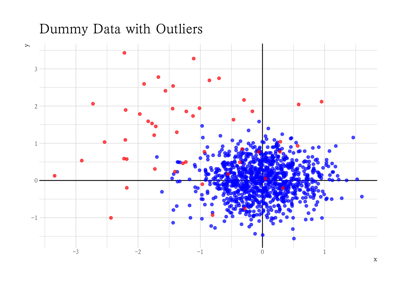
Dummy Data with Outliers
set.seed(1234)
N = 1e3
x = c(rnorm(N, 0, 0.5), rnorm(N * 0.05, -1, 1))
y = c(rnorm(N, 0, 0.5), rnorm(N * 0.05,  1, 1))
o = c(rep(0L, N), rep(1L, (N * 0.05)))
mm  <- matrix(x, y, nrow = N * 1.05, ncol = 2)
dat <- tibble(x, y, outlier = o)

dat |>
    ggplot(aes(x, y, col = factor(o))) +
    geom_vline(xintercept = 0) +
    geom_hline(yintercept = 0) +
    geom_point(alpha = 0.7) +
    scale_color_manual(values = c("0" = "blue", "1" = "red")) +
    guides(color = "none") +
    labs(title = "Dummy Data with Outliers")
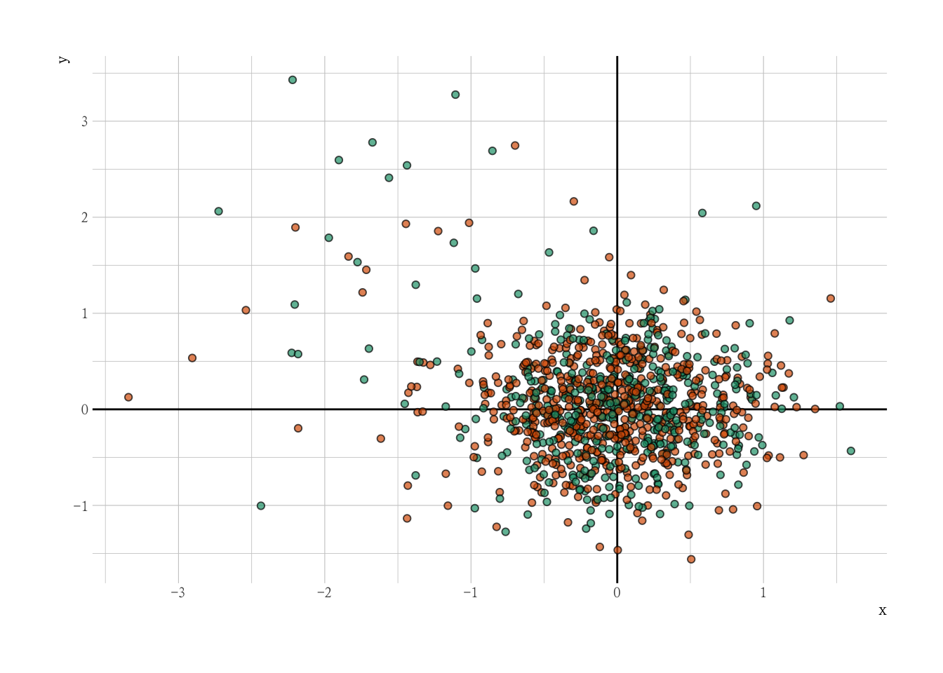
Kmeans-Clustering
既然我们知道了我们有两类数据组,离群值和非离群值,我们能不能利用聚类区分他们?
km <- kmeans(mm, centers = 2)

dat |>
    ggplot(aes(x, y, fill = factor(km$cluster))) +
    geom_vline(xintercept = 0) +
    geom_hline(yintercept = 0) +
    geom_point(alpha = 0.7, shape = 21, col = "black") +
    scale_fill_brewer(guide = "none", palette = "Dark2")
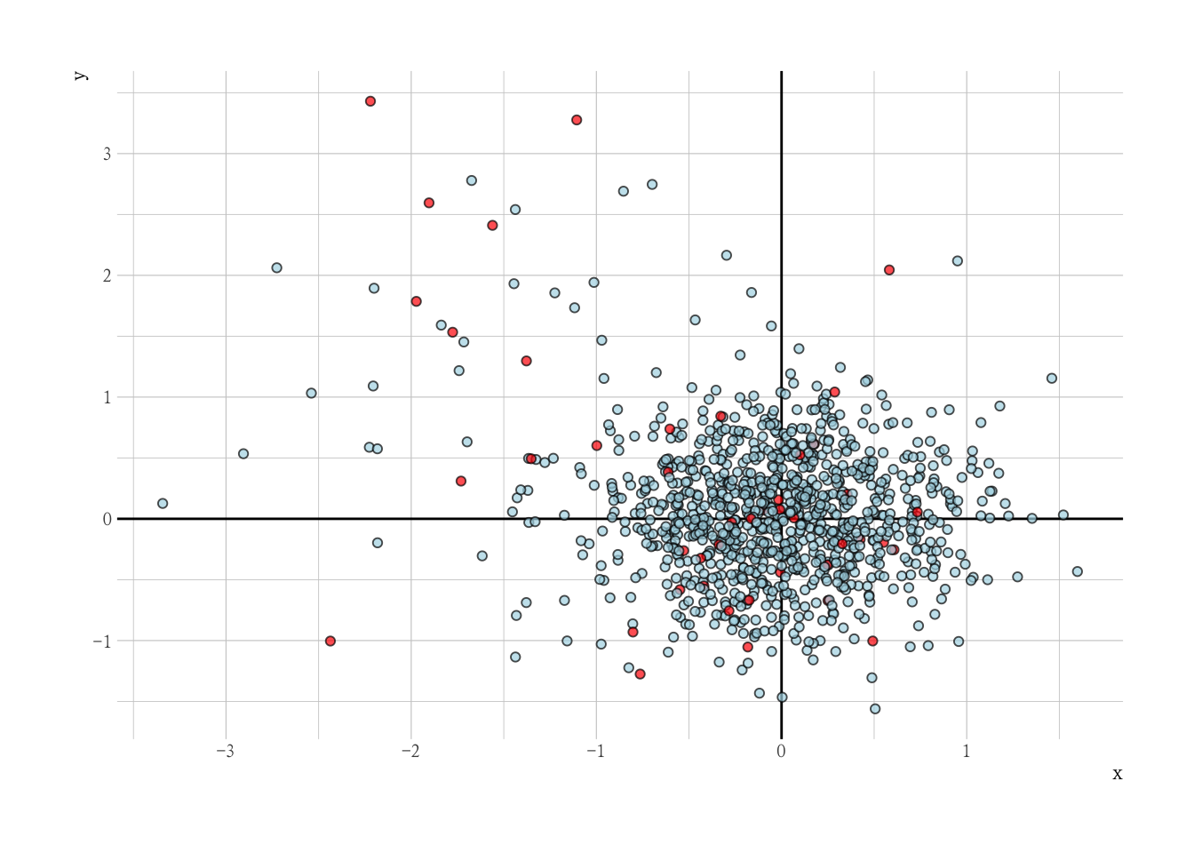
DBSCAN
DBSCAN 算法可以抽象为以下步骤:
- 找到每个点的 ε(eps)邻域中的点,并识别具有 m 个 (minPts) 邻居的核心点 (core points);
- 在邻居图上查找核心点的连通组件,忽略所有非核心点;
- 如果群集是 ε(eps)邻居,则将每个非核心点分配给附近的群集,否则将其分配给噪声;
library(dbscan)
# do density-based clustering
dbs <- dbscan(mm, eps = .3, minPts = 5, borderPoints = F)

dat |>
    ggplot(aes(x, y, fill = factor(dbs$cluster))) +
    geom_vline(xintercept = 0) +
    geom_hline(yintercept = 0) +
    geom_point(alpha = 0.7, shape = 21, col = "black") +
    scale_fill_manual(values = c("red", "lightblue")) +
    guides(fill = "none")
One-Class SVM
基本的原理就是利用 svm 进行单分类(正常类)
# One Class SVM ----------------------------------------------

library(e1071)

# nu is determined with hindsight over here
svmfit <- svm(mm, type = "one-classification", nu = 0.1)

dat |>
    mutate(is_outlier = predict(svmfit, mm)) %>%
    ggplot(aes(x, y, fill = factor(is_outlier))) +
    geom_vline(xintercept = 0) +
    geom_hline(yintercept = 0) +
    geom_point(alpha = 0.7, shape = 21, col = "black") +
    scale_fill_manual(values = c("red", "lightblue")) +
    guides(fill = "none")

Isolation Forest
孤立森林的核心假设是,异常数据只占很少量、且特征值和正常数据差别很大。因此如果使用递归地随机分割数据集,直到所有的样本点都是孤立的。在这种随机分割的策略下,异常点通常具有较短的路径。
library(solitude)

iso = isolationForest$new()
isofit <- dat |> select(-outlier) |> iso$fit()
## INFO  [21:35:06.549] Building Isolation Forest ...
## INFO  [21:35:06.981] done
## INFO  [21:35:06.984] Computing depth of terminal nodes ...
## INFO  [21:35:07.224] done
## INFO  [21:35:07.234] Completed growing isolation forest
dat |>
    bind_cols(iso$predict(dat)) |>
    mutate(is_outlier = anomaly_score > 0.65) |>
    ggplot(aes(
        x    = x,
        y    = y,
        fill = factor(-is_outlier)
    )) +
    geom_vline(xintercept = 0) +
    geom_hline(yintercept = 0) +
    geom_point(alpha = 0.7, shape = 21, col = "black") +
    scale_fill_manual(values = c("red", "lightblue")) +
    guides(fill = "none")
